Understanding Multiple Linear Regression in Machine Learning

Summary: Multiple linear regression is a statistical technique that models the relationship between one dependent variable and multiple independent variables. It is widely used in Machine Learning for predictions across various fields, employing a specific formula to analyse data effectively.

Introduction

Regression analysis in Machine Learning is a powerful tool for predicting outcomes based on input features. Among its various types, multiple linear regression stands out for its ability to model relationships between one dependent variable and two or more independent variables. 

Understanding the multiple linear regression formula is crucial for grasping how these relationships are quantified. This article will explore the fundamentals of multiple linear regression in Machine Learning, delve into a practical example, and illustrate how to apply the formula effectively. By the end, you’ll have a solid foundation in this essential technique.

What is Multiple Linear Regression?

Multiple linear regression is a statistical technique that models the relationship between one dependent variable and two or more independent variables. Unlike simple linear regression, which examines the relationship between two variables, multiple linear regression allows us to understand how various factors collectively influence the dependent variable. 

The goal is to find the best-fitting line or hyperplane that predicts the dependent variable based on the values of the independent variables.

Differences Between Simple and Multiple Linear Regression

The key difference between simple and multiple linear regression lies in the number of predictor variables used. Simple linear regression involves a single predictor to estimate the dependent variable, resulting in a straightforward line of best fit. 

In contrast, multiple linear regression incorporates multiple predictors, leading to a hyperplane in multidimensional space that fits the data. This approach provides a more nuanced understanding of how different factors interact and influence the outcome, offering a richer model for more complex datasets.

Applications in Machine Learning and Data Analysis

Multiple linear regression has applications in Machine Learning and Data Analysis. It is frequently used in finance to predict stock prices based on factors like interest rates and economic indicators. 

In healthcare, it helps predict patient outcomes based on various clinical parameters. Marketing analysts use it to understand how different marketing strategies affect sales. The technique is also helpful in real estate for estimating property values based on location, size, and other features.

Multiple linear regression provides valuable insights and predictive power by modelling complex relationships between variables, making it a fundamental tool in research and practical applications.

Read Blog: Anticipating Tomorrow: The Power of Predictive Modelling.

The Formula for Multiple Linear Regression

Multiple linear regression is a statistical method for modelling the relationship between a dependent variable and multiple independent variables. The formula for multiple linear regression is essential for understanding how changes in predictor variables influence the outcome. 

This formula helps predict the dependent variable based on the values of several independent variables. Let’s delve into the components of this formula to understand its structure and functionality.

Dependent Variable

In the multiple linear regression formula, the dependent variable, often denoted as y, represents the outcome or the variable we aim to predict. This variable depends on the independent variables and their respective coefficients. For instance, if we are predicting a house price, the house price is our dependent variable.

Independent Variables

The independent variables, denoted as x1,x2,…,xn​, are the predictors or features used to predict the value of the dependent variable. Each independent variable represents a different aspect or characteristic that may influence the dependent variable. For example, in predicting house prices, independent variables might include the number of bedrooms, location, and square footage.

Coefficients (Weights)

Coefficients, denoted as β1,β2,…,βn​, are the weights assigned to each independent variable. These coefficients measure the impact of each independent variable on the dependent variable. A higher coefficient value indicates a stronger relationship between the independent and dependent variables. For example, if β1​ is large, it means that changes in x1 have a significant effect on y.

Intercept

The intercept, denoted as β0​, represents the value of the dependent variable when all independent variables are equal to zero. It serves as the starting point of the regression line. In the context of our house price example, the intercept could represent the base price of a house with zero square footage and no additional features, although this scenario may be theoretical.

Mathematical Representation

The mathematical representation of the multiple linear regression formula is expressed as:

Here’s how each component fits into this equation:

• y: The predicted value of the dependent variable.
• β0​: The intercept of the regression line.
• β1,β2,…,βn​: The coefficients of the independent variables x1,x2,…,xn.
• x1,x2,…,xn​: The independent variables or predictors.
• ϵ: The error term or residual, accounting for the variability in y not explained by the independent variables.

Understanding the Formula

The formula combines all these elements to provide a linear equation that predicts the value of y. Each term βixi contributes to the overall prediction, with β0 setting the baseline. The error term ϵ adjusts for discrepancies between the predicted values and actual observations, ensuring the model accounts for random variations.

Analysing the formula and its components gives you insight into how multiple linear regression models work. This understanding is crucial for building effective predictive models and interpreting the relationships between variables in your data.

Also Check: An Introduction To Logistic Regression.

Assumptions of Multiple Linear Regression

Multiple linear regression relies on several key assumptions to produce accurate and reliable results. Understanding and checking these assumptions can help ensure that the model provides valid insights and predictions. Here are the primary assumptions of multiple linear regression:

Linearity

The relationship between the dependent variable and each independent variable must be linear. This means that changes in the independent variables should result in proportional changes in the dependent variable. Linear relationships allow the regression model to capture and accurately represent the data patterns.

Independence of Errors

The residuals (errors) should be independent. This implies that the error term for one observation should not be correlated with the error term for another observation. Independence is crucial for ensuring that the model’s predictions are not biased due to interdependencies in the data.

Homoscedasticity

The variance of the errors should remain constant across all levels of the independent variables. In other words, the spread of the residuals should be uniform across the range of predicted values. Homoscedasticity ensures that the model’s predictions are consistent and not skewed by varying error magnitudes.

Normality of Errors

The errors should be normally distributed. While this assumption is less critical for model estimation, it becomes essential for hypothesis testing and constructing confidence intervals. Normally distributed errors help in accurately assessing the reliability of the model’s coefficients.

No Multicollinearity

The independent variables should not be highly correlated. High multicollinearity can lead to unstable estimates of regression coefficients and make it difficult to determine the individual effect of each predictor on the dependent variable.

Ensuring these assumptions hold helps build a robust multiple linear regression model that can provide meaningful and actionable insights.

Example of Multiple Linear Regression

To illustrate how multiple linear regression works, let’s use a dataset to illustrate an example. The dataset contains information on various features that may influence a target variable. 

For this example, let’s consider a dataset containing information about houses. The goal is to predict house prices based on several features, such as the number of bedrooms, square footage, and the age of the house.Our dataset comprises several features:

• Number of Bedrooms: The count of bedrooms in the house.
• Square Footage: The total area of the house in square feet.
• Age of the House: The number of years since the house was built.
• Price: The target variable represents the price of the house in dollars.

We aim to build a multiple linear regression model to predict the house price based on the first three features.

Data Preparation

Before applying multiple linear regression, we need to prepare the data. Here’s a step-by-step breakdown:

• Cleaning the Data: Remove or impute missing values to ensure the dataset is complete.
• Encoding Categorical Variables: If any categorical variables are present, convert them into numerical form. In this example, our dataset is purely numerical.
• Feature Scaling: Standardise or normalise the features if they vary significantly in scale. This step ensures that all features contribute equally to the model.

Model Training

Model training in multiple linear regression involves using a dataset to estimate the relationships between independent variables and a dependent variable. This process optimises model parameters, allowing predictions and insights into data trends while minimising errors through techniques like gradient descent.With the data prepared, we can proceed to train the model:

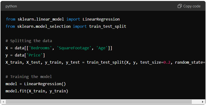
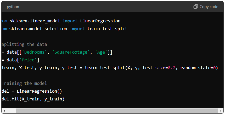
Splitting the Dataset: Divide the dataset into training and testing sets. A split of 80% training and 20% testing is typically used.

Fitting the Model: Use the training data to fit the multiple linear regression model. In Python, this can be done using libraries such as scikit-learn. For instance:

Evaluation of the Model

After training the model, evaluate its performance using the test data:

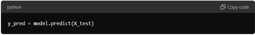
Predicting: Use the model to make predictions on the test set:

Metrics: Assess the model’s performance using metrics such as Mean Absolute Error (MAE), Mean Squared Error (MSE), and R-squared score. For example:

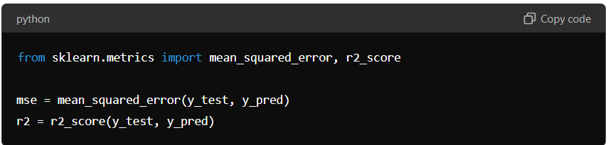
These metrics provide insights into how well the model predicts house prices. A lower MSE and a higher R-squared score indicate better performance.

Interpretation of Results

Interpreting the results involves analysing the coefficients and evaluating how well the model performs:

• Coefficients: Examine the regression model’s coefficients to understand each feature’s impact on the price. For example, a coefficient of 150 for square footage suggests that the price increases by $150 for every additional square foot.
• Model Performance: Consider the evaluation metrics. For instance, if the R-squared score is 0.85, the model explains 85% of the variance in house prices, indicating a good fit.

Visualisation

Visualisation can help to understand the model’s performance better:

• Scatter Plots: Create scatter plots to visualise the relationship between predicted and actual prices. This can help identify patterns or discrepancies.
• Residual Plots: Plot residuals to check for patterns that indicate issues with the model. Residuals should be randomly distributed.

In conclusion, by following these steps, you can effectively apply multiple linear regression to predict house prices and interpret the results to make informed decisions based on the model’s predictions.

Common Issues and How to Address Them

Several common issues can affect model performance and reliability when working with multiple linear regression. Understanding and addressing these issues is crucial for building accurate and robust models. Here’s a closer look at some typical challenges and strategies to manage them:

Overfitting and Underfitting

Overfitting occurs when a model learns the training data too well, capturing noise and the underlying pattern. This results in high accuracy on the training data but poor performance on new, unseen data. 

To combat overfitting, use techniques such as cross-validation, regularisation (like L1 and L2), and simplifying the model by reducing the number of features.

Underfitting happens when the model is too simple to capture the underlying trend in the data, leading to poor performance on both training and test sets. To address underfitting, consider adding more features, increasing the complexity of the model, or using more advanced algorithms.

Multicollinearity

Multicollinearity arises when the independent variables in the model are highly correlated. This can make it difficult to isolate each variable’s effect and lead to unstable coefficient estimates. 

To detect multicollinearity, check each predictor’s Variance Inflation Factor (VIF). Solutions include removing or combining correlated variables or using techniques like Principal Component Analysis (PCA) to reduce dimensionality.

Outliers and Influential Points

Outliers are data points that deviate significantly from other observations and can skew regression analysis results. Identify outliers using statistical tests or visualisation methods like scatter plots. Address them by verifying their validity, applying transformations, or using robust regression techniques.

Influential Points have a disproportionate impact on the model’s parameters. Evaluate influential points using measures like Cook’s distance. To manage these points, reassess their influence and consider whether they should be included in the model.

By proactively addressing these issues, you can enhance the accuracy and reliability of your multiple linear regression models.

Further Read About: 
Understanding Ridge Regression in Machine Learning.
Unlocking the Power of LASSO Regression: A Comprehensive Guide.

Closing Statements

Multiple linear regression is a vital tool in Machine Learning that enables the analysis of complex relationships between dependent and multiple independent variables. By understanding its formula and assumptions, practitioners can build predictive models that yield valuable insights across various fields, including finance, healthcare, and real estate. 

Mastering this technique allows data scientists to interpret results effectively and make informed decisions based on their analyses. As Machine Learning continues to evolve, the relevance of multiple linear regression remains significant, providing a foundation for more advanced modelling techniques.

Frequently Asked Questions

What is Multiple Linear Regression in Machine Learning?

Multiple linear regression is a statistical method to model the relationship between one dependent variable and two or more independent variables. It helps predict outcomes by determining how various factors collectively influence the dependent variable, making it essential for Data Analysis in Machine Learning.

Can you Provide a Multiple Linear Regression Example?

An example of multiple linear regression is predicting house prices based on features like the number of bedrooms, square footage, and house age. By analysing these independent variables, the model estimates the dependent variable, house price, using the multiple linear regression formula.

What is the Formula for Multiple Linear Regression?

The formula for multiple linear regression is expressed as:

y = β0 + β1×1 + β2×2 + … + βnxn + ϵ 

Here, y is the predicted value, β0 is the intercept, β1,β2,…,βn are the coefficients, x1,x2,…,xn are the independent variables, and ϵ is the error term.