Learning Exponential Smoothing for Time Series Forecasting

Summary: Exponential smoothing is a forecasting method using weighted averages of past data. It includes single, double, and triple methods for various data types, improving predictive accuracy for trends and seasonality. Learning and applying these methods can optimise forecasting in data analysis.

Introduction

It is a pivotal technique in time series forecasting, crucial for making predictions based on historical data. This blog delves into various methods, detailing their applications and formulas. Readers will learn about the method formula for simple, double, and triple, along with advanced variations like adaptive and seasonal smoothing. 

The objective is to equip data analysts with the knowledge to effectively implement exponential smoothing forecast formulas, enhancing their predictive accuracy. Whether you’re dealing with trends, seasonality, or intermittent demand, this guide provides comprehensive insights to optimise your forecasting endeavours.

What Is Exponential Smoothing?

This is a time series forecasting method for making predictions based on historical data. It assigns exponentially decreasing weights to past observations, with more recent observations receiving higher weights. 

It depends on a weighted average of past observations, making predictions for future data points.  The method formula for Simple Exponential Smoothing (SES), which is one of the most basic forms of exponential smoothing, is as follows:

Forecast for the next period (Ft+1):

Ft+1 = α * At + (1 – α) * Ft

Where:

• Ft+1 is the forecast for the next period (t+1).
• α (alpha) is the smoothing parameter, a value between 0 and 1 that determines the weight given to the most recent observation (At) versus the previous forecast (Ft). A higher α places more weight on the most recent observation.
• At is the actual value observed in the current period (t).
• Ft is the forecast made for the current period (t).

Types of Exponential Smoothing

This encompasses diverse methods tailored to various time series data and forecasting goals. Its versatility allows for tailored approaches, accommodating trends, seasonality, and adaptability to evolving patterns. Here, we delve into prevalent types, each uniquely adept at addressing distinct data characteristics and predictive needs.

Single Exponential Smoothing (SES)

SES is the simplest form of exponential smoothing. It is used for forecasting when the time series data does not exhibit a trend or seasonality. SES assigns exponentially decreasing weights to past observations, with a single smoothing parameter (alpha) controlling the weight assigned to the most recent observation.

Double Exponential Smoothing (Holt’s Linear Exponential Smoothing)

Double exponential smoothing extends SES by accounting for trends in time series data. It uses two smoothing parameters: alpha for level (similar to SES) and beta for trend. Use this method for time series data with a linear trend but no seasonality.

Triple Exponential Smoothing (Holt-Winters Exponential Smoothing)

Triple exponential smoothing extends double exponential smoothing to account for seasonality. It uses three smoothing parameters: alpha for level, beta for trend, and gamma for seasonality. This method is appropriate for time series data with both a trend and seasonality.

Seasonal Exponential Smoothing

Seasonal exponential smoothing is a variation of triple exponential smoothing. Use this method when the time series data has a significant seasonality component. It adjusts for seasonality by decomposing the data into level, trend, and seasonal components.

Adaptive Exponential Smoothing

Adaptive exponential smoothing modifies the smoothing parameters (alpha, beta, gamma) over time based on the data’s characteristics. This method is proper when the data’s underlying patterns change over time or when different periods require different levels of smoothing.

Exponential Smoothing with Damped Trends

Damped Trends incorporates a damping parameter to temper the trend component. This is particularly useful for modelling trends that gradually diminish over time rather than persist indefinitely. This addition enhances the model’s ability to reflect real-world scenarios where trends exhibit damping behaviour.

Exponential Smoothing with Box-Cox Transformation

Applying a Box-Cox transformation before exponential smoothing stabilises variances, mainly when data variances fluctuate over time. This method adjusts the data’s distribution, ensuring more consistent variance levels and enhancing exponential smoothing’s effectiveness in capturing underlying patterns and trends in the time series data.

Exponential Smoothing with Intermittent Demand Forecasting

Intermittent Demand Forecasting is tailored to predict sporadic demand, where specific periods exhibit zero or minimal demand. Approaches such as Croston’s method adapt the smoothing process to handle these irregularities, ensuring accurate forecasts despite intermittent demand patterns.

It depends on the characteristics of the time series data you are working with, including the presence of trends, seasonality, and the need for adaptability to changing patterns. Each type has advantages and limitations, so carefully analyse your data and forecasting objectives before selecting the most suitable method.

More For You To See:
5 Common Data Science Challenges and Effective Solutions.

Cheat Sheets for Data Scientists – A Comprehensive Guide.

13 Must Follow Best YouTube Channels for Data Science. 

How to Configure Exponential Smoothing

Configuring This involves determining the appropriate values for the smoothing parameters (alpha, beta, and gamma) and other settings based on your specific time series data and forecasting goals. Here’s a step-by-step guide:

Understand Your Data:

• Start by thoroughly understanding your time series data. Examine historical data to identify patterns, trends, and seasonality if present.
• Select the Exponential Smoothing Type:
• Choose the appropriate type of exponential smoothing based on your data’s characteristics. Consider whether your data exhibits a trend, seasonality, or both.

Choose an Initial Value for Smoothing Parameters:

• For Single Exponential Smoothing (SES), you only need to choose an initial value for the alpha parameter.
• For double exponential smoothing (Holt’s method), you must select initial alpha and beta values.
• For triple exponential smoothing (Holt-Winters method), you need initial alpha, beta, and gamma values.
• These initial values can be selected through trial and error, or you can use optimisation techniques to find the best values.

Determine the Seasonal Period (if applicable):

• If your data exhibits seasonality, determine the length of the seasonal period. 
• For example, if you have monthly data with a yearly seasonality pattern, the seasonal period is 12.

Split Your Data:

• Divide your historical data into a training set and a validation (or test) set. 
• The training set estimates the smoothing parameters, while the validation set assesses the forecasting accuracy.

Estimate the Smoothing Parameters:

• Use the training set to estimate the values of the smoothing parameters (alpha, beta, and gamma) for your chosen exponential smoothing method.
• You can use techniques like grid search, cross-validation, or optimisation algorithms to find the best parameter values that minimise the forecast error.

Apply Exponential Smoothing:

• After determining the optimal parameter values, apply the chosen ES forecast formula to your entire dataset, including the training and validation sets.

Validate and Evaluate the Model:

• Use the validation set to evaluate your model’s forecasting performance. Standard metrics for evaluation include Mean Absolute Error (MAE), Mean Squared Error (MSE), and Root Mean Squared Error (RMSE).
• Visualise the forecasted values alongside the actual data to assess how well the model captures the underlying patterns.

Refine and Tune the Model (if needed):

• If the forecasting performance is unsatisfactory, consider revisiting the parameter values or the chosen smoothing method.
• You may need to fine-tune the parameters to achieve better accuracy.

Implement the Configured Model:

• Once you are satisfied with the model’s performance on the validation set, you can use it to make future forecasts.

Monitor and Update the Model (if needed):

• Periodically reevaluate the model’s performance as new data becomes available. 
• You may need to adjust the smoothing parameters or other settings to account for changing patterns in the data.

Document Your Configuration:

• Record the selected smoothing parameters and any adjustments made over time. 
• This documentation will be valuable for maintaining and improving your forecasting model.

Configuring It is an iterative process that may require experimentation and fine-tuning to achieve accurate and reliable forecasts. When configuring the model, it’s essential to consider the specific characteristics of your data and the goals of your forecasting project.

Further Read:
What is Data Cleaning in Machine Learning?

Top ETL Tools: Unveiling the Best Solutions for Data Integration.

What is Data Scrubbing? Unfolding the Details.

Exponential Smoothing in Python

It is a popular method for time series forecasting, widely used in various domains such as finance, economics, and sales forecasting. In Python, implementing straightforward, leveraging libraries like pandas and stats models. Let’s delve into the process step by step.

Read More: 

Data Abstraction and Encapsulation in Python Explained.

Introduction to Model validation in Python.

Data Preparation

Before applying, it’s crucial to prepare your data adequately. It involves importing necessary libraries, loading the time series data into a pandas DataFrame, and ensuring the data is sorted chronologically.

To start:

• Import the required libraries, including pandas and stats models.
• Load your time series data into a pandas DataFrame.
• Ensure the data is sorted chronologically and convert it into a time series format if necessary.
• Choose the Model

The choice of the model depends on the characteristics of your data, such as trend and seasonality. Various variations of models are available, including Simple Exponential Smoothing (SES), Holt’s Linear Exponential Smoothing, and Holt-Winters Exponential Smoothing.

Consider the nature of your data and choose the appropriate model accordingly. For instance, SES might be suitable if your data exhibits a stable trend without seasonality. Holt-Winters Exponential Smoothing could be more relevant if your data has both trend and seasonality.

Parameter Estimation

Once you’ve chosen the model, the next step is to estimate the smoothing parameters based on your data. These parameters, such as alpha, beta, and gamma, control the level of smoothing applied to the data.

You can manually specify initial values for these parameters based on domain knowledge or use optimisation techniques to find the best parameters that minimise forecasting errors.

Apply Exponential Smoothing

With the model selected and parameters estimated, it’s time to apply ES to your time series data. The stats models library provides dedicated functions, making the implementation straightforward.

Utilise the chosen model and the estimated parameters to apply to your data. This process involves smoothing the data to capture underlying patterns effectively.

Generate Forecasts

After applying, you can generate forecasts for future periods using the fitted model. These forecasts provide insights into potential future trends and help in decision-making processes.

Utilise the fitted model to generate forecasts for future periods. These forecasts enable you to anticipate potential outcomes and plan accordingly.

Evaluate Model Performance

To assess the accuracy of your model, compare the forecasted values with the actual values. Various performance metrics, such as Mean Absolute Error (MAE) or Root Mean Squared Error (RMSE), can be calculated to evaluate the model’s performance.

Compare the forecasted values with the actual values to determine the accuracy of the model. Calculate performance metrics to quantify the level of accuracy and identify areas for improvement.

Visualise Results

Visualising the results of ES is essential for understanding how well the model captures the underlying patterns in the data. Time series plots displaying historical data and forecasted values provide valuable insights into the model’s effectiveness.

Create time series plots that showcase historical data along with forecasted values. Visualisation aids in interpreting the model’s performance and identifying any discrepancies between predicted and actual values.

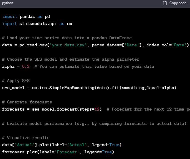
Here’s a simplified example of implementing Simple Exponential Smoothing (SES) in Python using the statsmodels library:

Frequently Asked Questions

What Is Exponential Smoothing In Time Series Forecasting?

It is a method for forecasting time series data. It assigns exponentially decreasing weights to past observations, with recent observations having more influence. This method helps predict future values based on historical data trends.

How Does The Exponential Smoothing Method Formula Work?

The simple ES formula is \( F_{t+1} = \alpha \cdot A_t + (1 – \alpha) \cdot F_t \), where \( \alpha \) is the smoothing parameter, \( A_t \) is the actual value, and \( F_t \) is the forecast. The formula weighs recent observations more heavily.

What Are The Types Of Exponential Smoothing Methods?

There are several types: Single Exponential Smoothing (SES) for data without trends, Double Exponential Smoothing for data with trends, and Triple Exponential Smoothing for data with trends and seasonality. Advanced types include adaptive, seasonal, and intermittent demand forecasting methods.

Conclusion

In conclusion, It is an effective method for conducting time series analysis. Data Analysts use this method to analyse historical data and make future predictions. 

As a Data Analyst aspirant, you must learn to conduct time series forecasting. You can become an expert by taking a Data Science foundational course by Pickl.AI to experience and learn Data Analytics skills.