Summary: Probability distributions are key in statistics. They show how random variable values are distributed. They aid in predicting outcomes and assessing risks, and types like Binomial, Normal, and Exponential commonly used.
Introduction
Probability distributions are fundamental in statistics. They represent how the values of a random variable distributed and provide a mathematical framework for predicting the likelihood of different outcomes, making them essential for data analysis.
Understanding probability distributions allows statisticians and analysts to interpret data patterns, assess variability, and make informed decisions based on statistical evidence. This article explores the concept of probability distributions, highlights their key features, and discusses their importance in various real-world applications.
By the end, you’ll clearly understand how probability distributions influence data-driven decisions.
Read Blog:
Statistical Tools for Data-Driven Research.
An Introduction to Statistical Inference.
What is a Probability Distribution?
A Probability Distribution provides a mathematical function that links each possible outcome of a random variable to its corresponding probability. A probability mass function (PMF) represents the probability distribution for a discrete random variable.
In contrast, a probability density function represents a continuous random variable (PDF). In both cases, the distribution must satisfy two fundamental properties: the probabilities of all outcomes must sum to 1, and each probability must be between 0 and 1.
Explanation of Probability Distribution
Understanding Probability Distributions is crucial because they provide a comprehensive picture of a random variable’s behaviour. Knowing the probability distribution, one can calculate various statistical measures such as the mean, variance, and standard deviation, which help summarise the data and make predictions.
For instance, if you know the probability distribution of a company’s monthly sales, you can predict future sales, assess the risk of low sales months, and make informed decisions about inventory and staffing.
Probability distributions also play a crucial role in hypothesis testing, where they help determine whether observed data deviates significantly from what is expected.
Examples to Illustrate the Concept
- Coin Toss: Consider the simple example of tossing a fair coin. The random variable here is the outcome of the toss, which can be heads or tails. The probability distribution assigns a probability of 0.5 to both heads and tails since both outcomes are equally likely.
- Rolling a Die: When rolling a six-sided die, the random variable is the number that comes up. The probability distribution for this event is uniform, as each outcome (1 through 6) has an equal probability of 1/6.
- Normal Distribution: The height of individuals in a large population often follows a normal distribution. In this continuous distribution, most individuals have heights around the mean, with fewer individuals at the extremes (very short or tall). The normal distribution characterised by its bell-shaped curve, where the probability of outcomes closer to the mean is higher.
Explore More:
A Comprehensive Guide to Descriptive Statistics.
Crucial Statistics Interview Questions for Data Science Success.
Inferential Statistics to Boost Your Career in Data Science.
Key Features of Probability Distributions

Understanding the key features of probability distributions is crucial for interpreting data and making informed decisions. These features provide insights into a distribution’s central tendency, variability, and shape. This section will explore these features in detail, with explanations, formulas, and examples.
Mean (Expected Value)
The mean, the expected value, is the central measure of a probability distribution. It represents the average outcome that one can expect from a random variable if the experiment repeated many times. The mean calculated by multiplying each possible value of the random variable by its probability and then summing these products.
Significance:
The mean is a fundamental measure in probability and statistics. It provides a single value summarising the entire distribution, making it easier to compare different distributions. For example, the mean score indicates the student’s overall performance in a distribution of test scores.
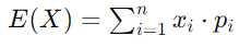
Calculation Method:
For a discrete random variable X with possible values x1,x2,…,xn and corresponding probabilities p1,p2,…,pn, the mean E(X) is calculated as:
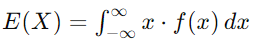
For a continuous random variable, the mean calculated using the integral of the product of the variable and its probability density function f(x):
Example:
Consider a fair six-sided die. The possible outcomes are 1, 2, 3, 4, 5, and 6, each with a probability of 1/6. The mean of this distribution is:

Variance and Standard Deviation
Variance measures the spread or variability of a probability distribution. It indicates how much the values of the random variable deviate from the mean. The standard deviation, the square root of the variance, measures this spread in the same units as the original data.
Explanation of Variability:
High variance indicates that the data points are spread out over a wide range of values, while low variance suggests that the data points clustered close to the mean.
Formulas:
For a discrete random variable, the variance Var(X) is calculated as:

Where μ is the mean of the distribution.
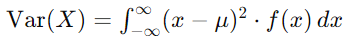
For continuous random variables:
Example:
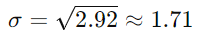
Using the die example, the variance is calculated as:

The standard deviation is:
Skewness
Skewness measures the asymmetry of a probability distribution around its mean. It indicates whether the distribution has a longer tail on the left (negative skew) or right (positive skew).
Types of Skewness:
- Positive Skew: The tail on the right side is longer, and the bulk of the data is on the left. The mean is greater than the median.
- Negative Skew: The tail on the left side is longer, and most of the data is on the right. The mean is less than the median.
Example:
An example of positive skewness is income distribution, where many individuals earn significantly more than the majority, stretching the tail to the right.
Kurtosis
Kurtosis describes the “tailedness” of a probability distribution. It measures the height and sharpness of the peak relative to a normal distribution.
Types of Kurtosis:
- Leptokurtic: Distributions with sharp peaks and fat tails. These have a higher kurtosis than normal distributions.
- Platykurtic: Distributions with flat peaks and thin tails, indicating lower kurtosis.
- Mesokurtic: Distributions that resemble a normal distribution with moderate kurtosis.
Relevance:
Kurtosis is crucial in risk management and financial modelling, where extreme values (outliers) can significantly impact.
Probability Density Function (PDF) and Cumulative Distribution Function (CDF)
The Probability Density Function (PDF) describes the relative likelihood of a continuous random variable taking a particular value+, while the Cumulative Distribution Function (CDF) represents the probability that the random variable is less than or equal to a given value.
The Probability Density Function (PDF) describes the likelihood of a random variable taking a specific value. It’s the function that defines the shape of the distribution. For a continuous random variable, the area under the curve of the PDF represents the probability of the variable falling within a specific range.
CDF
The Cumulative Distribution Function (CDF) gives the probability that a random variable is less than or equal to a specific value. It derived by integrating the PDF and provides a cumulative probability measure.
Example
The PDF bell-shaped for a standard normal distribution, and the CDF smoothly transitions from 0 to 1, indicating the cumulative probability up to any given point on the distribution.
Check: Exploring The Top Key Statistical Concepts.
Common Types of Probability Distributions

Probability distributions can broadly categorised into two types: discrete and continuous. This section will explore some of the most common probability distributions, their definitions, key features, and practical use cases.
Discrete Distributions
Discrete probability distributions describe scenarios where the set of possible outcomes is countable. Each outcome has a specific probability associated with it. Two of the most widely used discrete distributions are the Binomial and Poisson distributions.
Binomial Distribution
The Binomial Distribution models the number of successes in a fixed number of independent trials, where each trial has two possible outcomes—success or failure. The probability of success remains constant across all trials. The distribution defined by the number of trials (n) and the probability of success in a single trial (p).
Features
- Binary Outcomes: Each trial has only two possible outcomes, often labelled as “success” and “failure.”
- Fixed Number of Trials: The number of trials, n, is predetermined.
- Independent Trials: One trial’s outcome does not influence another’s outcome.
- Constant Probability: The probability of success, p, remains the same for all trials.
- Shape: Depending on the values of n and p, the binomial distribution can be symmetric or skewed.
Use Cases
The Binomial Distribution commonly used in scenarios where you must determine the probability of a specific number of successes in a series of trials. Examples include:
- Quality Control: Assessing the probability of certain defective items in a batch.
- Marketing: Evaluating the likelihood of a specific number of customers purchasing a marketing campaign.
- Medical Studies: Estimating the probability of a certain number of patients responding positively to a treatment.
Poisson Distribution
The Poisson Distribution models the number of times an event occurs within a fixed interval of time or space, assuming that the events occur independently and with a constant average rate. The distribution is defined by a single parameter, λ (lambda), representing the average number of occurrences within the interval.
Features
- Event Occurrence: The Poisson Distribution focuses on the number of occurrences of an event within a specified interval. Use poisson distribution calculator to find the number of occurrences of any event.
- Independent Events: The occurrence of one event does not affect the occurrence of another.
- Constant Rate: The average rate of occurrence, λ, is continuous.
- No Upper Limit: The number of occurrences can theoretically be infinite, though higher numbers become increasingly improbable.
Use Cases
The Poisson Distribution is often applied when you are interested in the frequency of events occurring over a continuous interval. Examples include:
- Call Centers: Estimating the number of incoming calls in a given hour.
- Traffic Analysis: Predicting the number of cars passing through a toll booth daily.
- Healthcare: Modeling the number of patients arriving at an emergency room during a shift.
Continuous Distributions
Continuous probability distributions describe outcomes that can take any value within a specified range. Unlike discrete distributions, which deal with countable outcomes, continuous distributions deal with uncountable outcomes. The most common continuous distributions include the Normal, Exponential, and Uniform Distributions.
Normal Distribution
The Normal Distribution, also known as the Gaussian Distribution, is a continuous, symmetrical, bell-shaped probability distribution. It is defined by the mean (μ) and the standard deviation (σ). The mean determines the centre of the distribution, while the standard deviation controls the spread.
Features
- Symmetry: The distribution is perfectly symmetrical around the mean.
- Mean, Median, and Mode: In a normal distribution, the mean, median, and mode are all equal.
- 68-95-99.7 Rule: Approximately 68% of the data falls within one standard deviation of the mean, 95% within two, and 99.7% within three.
- Tails: The tails of the distribution approach the horizontal axis asymptotically, never touching it.
Importance
The Normal Distribution is one of the most important statistical distributions, as many natural phenomena and measurement errors tend to follow this pattern. It is widely used in hypothesis testing, regression analysis, and quality control.
Use Cases
- Psychology: IQ scores are often modelled using a normal distribution.
- Finance: Stock market returns are frequently assumed to follow a normal distribution.
- Manufacturing: Product dimensions in quality control often adhere to a normal distribution.
Exponential Distribution
The Exponential Distribution is a continuous probability distribution that models the time between events in a Poisson process, where events occur continuously and independently at a constant average rate. It is defined by a single parameter, λ (lambda), the rate parameter.
Features
- Memoryless Property: The exponential distribution has the memoryless property, meaning the probability of an event occurring in the future is independent of past events.
- Asymmetry: The distribution is right-skewed, with a long tail extending to the right.
- Rate Parameter: The rate parameter, λ, inversely determines the average time between events.
Use Cases
The Exponential Distribution is often used in scenarios involving waiting times between events. Examples include:
- Queuing Theory: Modeling the time between arrivals of customers at a service centre.
- Reliability Engineering: Estimating the time until a system or component fails.
- Telecommunications: Predicting the time between incoming phone calls at a call centre.
Uniform Distribution
The Uniform Distribution is a continuous probability distribution where all outcomes are equally likely within a specified range [a, b]. The probability density function is constant, and the distribution is defined by two parameters: the minimum value (a) and the maximum value (b).
Features
- Equally Likely Outcomes: Every outcome within the specified range has the same probability.
- Rectangular Shape: The probability density function forms a rectangle, as the probability is constant.
- Finite Range: The distribution is only defined within the interval [a, b], and no outcomes can occur outside this range.
Use Cases
The Uniform Distribution is commonly used in situations where each outcome within a range is equally likely. Examples include:
- Random Number Generation: Generating random numbers within a specified range.
- Simulation: Modeling scenarios where all outcomes in a range are equally probable.
- Decision Making: Assigning equal probabilities to multiple options in a decision-making process.
This overview of common probability distributions, including their definitions, features, and use cases, provides a foundational understanding essential for statistical analysis and data modelling. Each distribution serves unique purposes and is applied in various fields to interpret and predict real-world phenomena.
Also Check: Most Popular Statistician Certification For Your Success.
Importance of Probability Distributions

Probability distributions provide a framework for understanding the likelihood of different outcomes and allow us to make informed decisions based on data. We can predict future events, assess risks, and model complex systems by analysing probability distributions. Here’s why probability distributions are crucial:
Predictive Analysis
Probability distributions enable predictive analysis by helping us estimate the likelihood of future events. By understanding the distribution of past data, we can forecast potential outcomes and trends. For example, businesses use probability distributions to predict sales, stock prices, or customer behaviour, allowing them to plan strategically.
Decision Making
Informed decision-making relies heavily on understanding probability distributions. When faced with uncertainty, knowing the distribution of possible outcomes allows decision-makers to weigh risks and benefits. This insight leads to more rational and evidence-based business, finance, or everyday choices.
Risk Assessment
Probability distributions play a vital role in assessing and managing risks. Organisations can identify and quantify risks by analysing the distribution of potential losses or failures. This information is critical in industries like insurance, finance, and engineering, where understanding risk is essential for creating effective mitigation strategies.
Data Modelling
Probability distributions are indispensable in statistical modelling and simulation. They provide the mathematical foundation for creating models that simulate real-world processes. Whether in machine learning, econometrics, or scientific research, probability distributions help make accurate and reliable models that predict outcomes and inform decisions.
Explore More:
Exploring 5 Statistical Data Analysis Techniques with Real-World Examples.
Different Types of Statistical Sampling in Data Analytics.
How can you become a statistician without a degree?
Closing Statements
Probability distributions are foundational in statistics, offering a framework to understand and predict random variables’ behaviour. They enable effective decision-making, risk assessment, and data modelling across various fields. Analysts and researchers can gain valuable insights and make informed predictions based on data by grasping different distributions.
Frequently Asked Questions
What are Probability Distributions?
Probability distributions represent how the values of a random variable are spread out. They provide functions that link each possible outcome to its probability, helping to predict the likelihood of various results. This concept is essential for data analysis and statistical modelling.
Why are Probability Distributions Important?
Probability distributions are vital for making informed decisions, assessing risks, and predicting future events. Organisations and researchers can model uncertainties, forecast trends, and implement effective financial, healthcare, and engineering strategies by understanding data distribution.
What are Common Types of Probability Distributions?
Common probability distributions include the Binomial (for success/failure outcomes), Poisson (for event counts), Normal (a bell-shaped curve), Exponential (time between events), and Uniform (equal probability within a range). Each distribution serves unique purposes and is used in different data analysis scenarios.
Authors
-

Written by:
Smith AlexReviewed by: