Exploring The Top Key Statistical Concepts 

Summary: Statistical analysis is the key to unlocking the secrets hidden within your data. For any individual who wants to become a proficient Data Scientist, mastering the Data Science skills is imperative. Statistics for Data Science is the fundamental skill set that helps a Data Scientist complete their tasks with accuracy.

Statistics for Data Science: Exploring The Top Key Statistical Concepts

Data Science thrives on the ability to extract meaningful insights from vast amounts of data. Statistics for Data Science forms the backbone of this process, providing a framework for analyzing, interpreting, and drawing conclusions from information.

This article explores five key statistical concepts that are fundamental for any aspiring Data Scientist. These are a must-know Data Science skills that boosts your profile and enhances work efficiency. 

Probability and Probability Distributions

Probability refers to the likelihood of an event occurring. It’s expressed as a number between 0 (impossible) and 1 (certain). Probability distributions describe the range of possible values for a variable and the likelihood of each value occurring.

Common distributions include the normal distribution (bell curve), used for continuous data like height, and the binomial distribution, used for events with two possible outcomes (e.g., success/failure).

Example

A Data Scientist analyzing online customer reviews might use a binomial distribution to understand the probability of a positive review.

Scenario

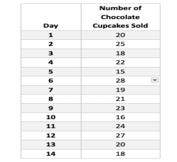
A bakery monitors its daily cupcake sales to understand customer preferences and optimize production. They record sales data for chocolate cupcakes over a two-week period (14 days), resulting in the following figures:

Data Analysis: Probability and Probability Distribution

Calculate Probability of Selling a Specific Number of Cupcakes:

For instance, let’s calculate the probability of selling exactly 20 chocolate cupcakes on a given day.

• We know the total number of observations (days) is 14.
• Favorable outcome (selling 20 cupcakes) occurred twice (on Day 1 and Day 13).

Therefore, the probability of selling 20 cupcakes:

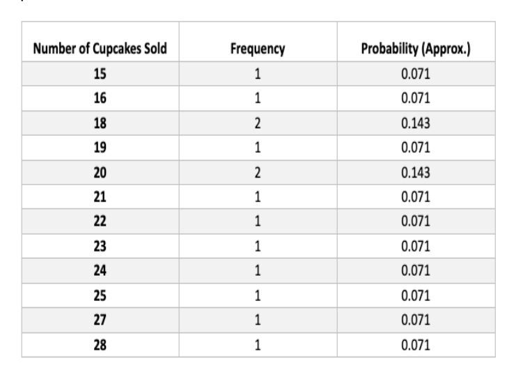
Probability (selling 20) = Favorable outcomes / Total outcomes = 2 / 14 ≈ 0.143

Analyze Probability Distribution

We can analyze the probability distribution of daily cupcake sales by calculating the frequency of each number sold. Here’s a table summarizing the results:

Visualization with Histogram

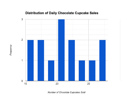
By plotting a histogram, we can visualize the probability distribution of the data. The histogram shows the frequency of each number of cupcakes sold on the x-axis and the frequency count on the y-axis.

Applications

Probability and probability distributions are crucial for tasks like predicting future outcomes, assessing risk, and designing A/B tests to compare website variations.

Descriptive Statistics

Descriptive statistics summarize the key characteristics of a dataset. This includes measures of central tendency (mean, median, mode) that indicate the “average” value, and measures of variability (range, standard deviation) that describe how spread out the data is.

Example

A Data Scientist studying house prices in a city might calculate the mean, median, and standard deviation of the prices to understand the typical price range and the level of variation within that range.

Scenario

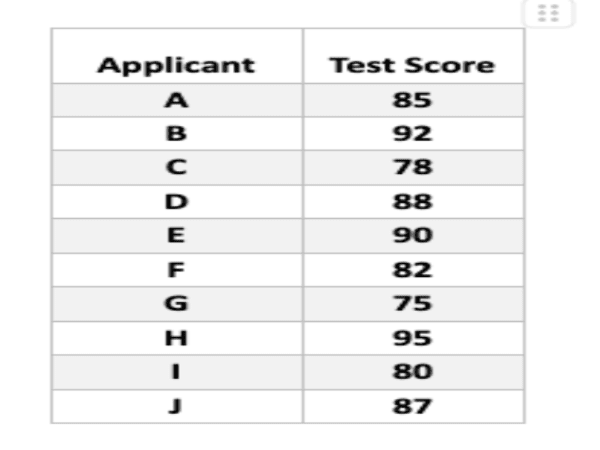
Imagine a company tracks the test scores of 10 new software developer applicants. Here’s the data:

We can use various measures to summarize this data set:

Measures of Central Tendency

Mean: This represents the average score. Add all scores and divide by the number of applicants (n = 10).

Mean = (85 + 92 + 78 + 88 + 90 + 82 + 75 + 95 + 80 + 87) / 10 = 85.2

Median: This is the “middle” score when arranged in ascending order.

75, 78, 80, 82, 85, 87, 88, 90, 92, 95

Median = (85 + 87) / 2 = 86

Mode: This is the most frequent score. In this case, there isn’t a single most frequent score.

Measures of Variability

Range: This represents the difference between the highest and lowest scores.

Range = 95 – 75 = 20

Standard Deviation: This measures how spread out the data is from the mean. Calculating the standard deviation involves more complex steps, but online tools can help.

Interpretation

Looking at the measures of central tendency, the mean and median suggest most scores fall around the mid-80s range. There isn’t a single most frequent score (mode). The range of 20 indicates some variation in scores, but the standard deviation would provide a more precise measure of this spread.

Applications

Descriptive statistics provide a quick overview of the data, allowing Data Scientists to identify trends, outliers, and potential areas for further investigation.

Hypothesis Testing

Hypothesis testing is a statistical method to assess the validity of a claim (hypothesis) about a population based on a sample of data. It involves formulating a null hypothesis (no difference exists) and an alternative hypothesis (a difference exists), and then conducting a statistical test to determine if the evidence supports rejecting the null hypothesis.

Example

A marketing team believes a new social media campaign will increase website traffic. They run a hypothesis test to determine if the observed increase in traffic after launching the campaign is statistically significant, meaning it’s unlikely to be due to chance.

Plant Growth and Fertilizer: A Hypothesis Test

Let’s say a botanist wants to investigate if a new fertilizer increases plant growth. Here’s a numerical example of hypothesis testing:

Scenario

We measure the heights (in centimeters) of 10 randomly chosen tomato plants (sample size, n=10) that haven’t received the new fertilizer. We want to see if there’s evidence to suggest the average plant height (population mean, μ) is greater than 20cm after using the fertilizer.

Step 1: Define the Hypotheses

• Null Hypothesis (H₀): μ ≤ 20cm. There’s no significant difference in plant height with or without fertilizer (average height is 20cm or less).
• Alternative Hypothesis (H₁): μ > 20cm. The new fertilizer increases plant height (average height is greater than 20cm).

Step 2: Choose Significance Level (α)

Let’s set the significance level (α) at 5%. This means we’re willing to risk a 5% chance of rejecting the null hypothesis when it’s actually true (a type I error).

Step 3: Collect Sample Data

Suppose we measure the heights of 10 tomato plants that received the new fertilizer and get the following data (in centimeters):

23, 25, 21, 27, 22, 24, 28, 20, 26, 29

Step 4: Calculate Sample Mean (x̄)

Average the heights: x̄ = (23 + 25 + 21 + … + 29) / 10 = 24.8 cm

Step 5: Perform the Statistical Test

Since our sample size (n) is less than 30 and the population standard deviation (σ) is unknown, we’ll use a t-test.

• Calculate the t-statistic (assuming equal variances):

t = (x̄ – μ₀) / (s / √n)

Here:

• x̄ = sample mean (24.8 cm)
• μ₀ = value from the null hypothesis (20 cm)
• s = sample standard deviation (we’ll need to calculate this from the sample data)
• √n = square root of sample size (√10)

Step 6: Make a Decision (Critical Value)

• Look up the critical t-value for a two-tailed test with α = 0.05 and degrees of freedom (df) = n-1 = 9. (You can find t-value tables online).
• If the calculated t-statistic (t) is greater than the critical t-value, reject H₀. This suggests evidence for the alternative hypothesis (increased plant height).
• If the calculated t-statistic (t) is less than the critical t-value, fail to reject H₀. There isn’t enough evidence to conclude the fertilizer definitively affects plant height.

Applications

Hypothesis testing is essential for making informed decisions based on data. It helps Data Scientists differentiate between random fluctuations and genuine effects.

Correlation and Regression Analysis

Correlation measures the strength and direction of the linear relationship between two variables. A positive correlation indicates values of one variable tend to increase with the other, while a negative correlation indicates they tend to move in opposite directions. Regression analysis builds on correlation, but it aims to predict the value of one variable (dependent variable) based on another variable (independent variable).

Example

A Data Scientist analyzing retail sales data might find a positive correlation between online advertising spending and customer traffic in stores. Regression analysis could then be used to predict store traffic based on planned advertising expenditure.

Numerical Example: Studying Hours and Exam Scores

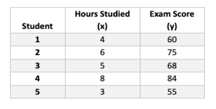
Let’s say we’re investigating the relationship between the number of hours spent studying (independent variable, x) and exam scores (dependent variable, y) for a small group of students.

Here’s a table with some example data:

We can calculate the correlation coefficient (r) to measure the strength and direction of the linear relationship between studying hours and exam scores. There are different correlation coefficients, but a common one for continuous data is Pearson’s correlation coefficient.

Using a calculator or statistical software, we find r = 0.87 for this data set.

Interpretation

• Positive correlation (r = 0.87): There’s a positive association between studying hours and exam scores. As students study more, their scores tend to go up.
• Strength of correlation (r close to 1): The value of 0.87 is relatively high, indicating a strong positive correlation.

Regression Analysis

Regression analysis helps us find an equation to represent the relationship between the variables. In this case, we’re looking for a linear equation to predict exam scores (y) based on studying hours (x).

Using linear regression, we get an equation like this (example formula, actual coefficients may vary):

y = 5 + 8.5x

Interpretation

• The y-intercept (5) represents the predicted exam score when students study for 0 hours (which wouldn’t be realistic, but it helps with the equation).
• The slope (8.5) indicates that for every additional hour studied, the predicted exam score increases by 8.5 points on average.

Applications

Correlation and regression analysis are invaluable tools for understanding relationships between variables and making predictions. They can be used to identify trends, develop marketing strategies, and optimize business operations.

Sampling and Sampling Techniques

Rarely can Data Scientists analyze an entire population (all possible data points). Instead, they rely on samples – a subset of the population that is used to make inferences about the whole. Choosing the right sampling technique is crucial for ensuring the sample accurately represents the population.

Common techniques include random sampling (each member has an equal chance of being selected), stratified sampling (ensures subgroups within the population are adequately represented), and cluster sampling (groups of individuals are chosen instead of individual observations).

Example

A Data Scientist studying customer satisfaction wants to survey a representative sample of the company’s customer base. They might choose a stratified sampling technique to ensure the survey includes a proportional number of customers from different age groups and geographical locations.

Numerical Example: Sampling Techniques in a Bakery

Let’s say a bakery owner wants to understand customer preferences for their cupcakes. They have a record of 100 customers who bought cupcakes in the last week.

Population: All 100 customers of the bakery in the last week.

Sample Size: We want to survey 20 customers.

Sampling Technique 1: Simple Random Sampling

Assign Numbers: Assign a unique number (1-100) to each customer on the record.

Random Selection: Use a random number generator to pick 20 unique numbers between 1 and 100.

Survey: Survey the customers corresponding to the chosen numbers.

This ensures each customer has an equal chance of being selected, providing an unbiased sample.

Sampling Technique 2

Stratification: Knowing cupcake preferences might differ by age, the bakery owner divides the customers into two age groups (20-35 & 36-55) with 60 and 40 customers respectively.

Proportional Selection: Since the age groups are not equal, proportional sampling is used. We need to select 12 customers from the younger group (60% of 20) and 8 customers from the older group (40% of 20).

Random Selection Within Groups: Use random number generation to pick 12 customers from the younger group and 8 from the older group.

Survey: Survey the selected customers from each age group.

This ensures the sample reflects the age distribution of the customer base, providing a more targeted view of preferences.

Applications

Understanding sampling and sampling techniques is vital for drawing valid conclusions from data. It helps to avoid bias and ensures that findings can be reliably generalized to the broader population.

Frequently Asked Questions

What’s The Difference Between Population and Sample in Data Science?

Data Scientists often analyze samples because studying the entire population can be impractical or expensive.  Understanding the difference helps ensure your conclusions about the population are accurate.

Population: The entire collection of individuals or items you’re interested in studying. Imagine it as all the cookies in a bakery.

Sample: A smaller group chosen to represent the entire population. It’s like grabbing a handful of cookies from the bakery to understand the overall flavor profile.

What Are Descriptive Statistics Good For?

Descriptive statistics  summarize the key characteristics of your data. They’re like giving a brief description of your handful of cookies. For example, you might  calculate the average size (mean), how many chocolate chip cookies there are (frequency), or the spread of sizes (standard deviation).

Descriptive statistics help you understand the basic properties of your data and identify potential patterns or trends.  

What’s The Benefit of Using Hypothesis Testing in Data Science?

Hypothesis testing allows you to make informed guesses about the population based on your sample. Like wondering if the bakery uses a standard cookie cutter based on the similar sizes in your handful.

You set up a hypothesis (e.g., “all cookies are the same size”) and then use statistical tests to see if the sample data supports it  (strong evidence) or suggests otherwise (weak evidence). This helps Data Scientists draw reliable conclusions that go beyond just describing the sample itself. 

Concluding Remarks

These five key statistical concepts are just the foundation. Data Science is a rapidly evolving field with numerous advanced statistical methods.

However, a strong understanding of these core concepts will equip you to analyze data effectively, identify patterns, and extract valuable insights that can drive informed decision-making. 

To start your learning journey in Data Science, you can enroll for the Data Science course that will equip you with the right Data Science skills and tools. Pickl.AI offers a perfect learning platform for all tech neophytes as well as professionals. To learn more about the Data Science course, log on to pickl.ai today.