All About the Empirical Formula In Statistics

Summary: The empirical Formula or the 68-95-99.7 rule, is a fundamental concept in statistics that describes how data is distributed in a normal distribution. It states that approximately 68% of data falls within one standard deviation of the mean, 95% within two standard deviations, and 99.7% within three standard deviations. This rule is widely applicable in various fields such as finance, healthcare, and education for making predictions and assessing probabilities.

Introduction

The empirical rule, often referred to as the “68-95-99.7 rule” or the “three-sigma rule,” is a fundamental concept in statistics that describes how data is distributed in a normal distribution.

This rule is essential for statisticians and Data Analysts as it provides a quick way to understand the spread of data points around the mean.

In this blog, we will delve into the empirical rule, its significance, applications, limitations, and provide illustrative examples to enhance understanding.

Key Takeaways

• The empirical rule applies to normally distributed data for accurate predictions.
• Approximately 68% of data lies within one standard deviation of the mean.
• About 95% of data falls within two standard deviations from the mean.
• Nearly all (99.7%) data is contained within three standard deviations.
• It is crucial for quality control and risk management across industries.

Understanding the Empirical Rule

The empirical rule states that for a normal distribution:

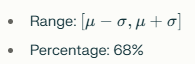
• Approximately 68% of the data falls within one standard deviation of the mean (μ±σμ±σ).
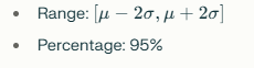
• About 95% of the data lies within two standard deviations (μ±2σμ±2σ).
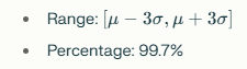
• Nearly 99.7% of the data is contained within three standard deviations (μ±3σμ±3σ).

This distribution creates a bell-shaped curve when graphed, with the mean at the centre. The empirical rule is particularly useful because it allows statisticians to make inferences about a dataset without needing to examine every individual data point.

Graphical Representation

To visualise the empirical rule, imagine a bell curve where:

• The peak represents the mean of the dataset.
• The area under the curve represents the total probability (which equals 1 or 100%).

The standard deviations are marked along the x-axis:

• One standard deviation on either side of the mean captures 68% of all data points.
• Two standard deviations capture 95%.
• Three standard deviations capture 99.7%.

This visual representation helps in understanding how concentrated data points are around the mean and how they taper off as you move away from it.

Mathematical Formulation

The empirical rule can be mathematically expressed using the mean (μμ) and standard deviation (σσ) of a dataset:

One standard deviation

Two standard deviations

Three standard deviations:

This formula allows statisticians to predict how much of their data will fall within these ranges based on calculated mean and standard deviation values.

Application of Empirical Rule

The empirical rule, also known as the 68-95-99.7 rule, is a statistical principle that describes how data distributed in a normal distribution. This rule is widely applicable across various fields, helping professionals make informed decisions based on the distribution of data. Below are some key applications of the empirical rule in different sectors:

Finance and Accounting

In finance, the empirical rule is crucial for forecasting and risk management. Financial analysts use it to assess the volatility of stock prices and investment returns. 

By understanding that approximately 68% of returns will fall within one standard deviation of the mean, analysts can better predict potential gains or losses. This insight helps in setting realistic profitability goals and managing investment risks effectively.

Marketing Analytics

Marketing professionals leverage the empirical rule to evaluate campaign performance and consumer behaviour. By analysing historical data on customer interactions and engagement metrics, marketers can determine expected ranges for future campaigns. 

For instance, if past campaign engagement follows a normal distribution, they can use the empirical rule to estimate how many customers are likely to respond positively to new marketing strategies, allowing for better resource allocation.

Healthcare

In healthcare, the empirical rule aids in analysing patient data and predicting health outcomes. Medical researchers often use it to assess the effectiveness of treatments or medications by examining patient recovery rates. 

For example, if recovery times for a specific treatment follow a normal distribution, healthcare providers can apply the empirical rule to estimate the likelihood of different recovery times among patients, enhancing treatment planning and resource allocation.

Education

The education sector employs the empirical formula statistics to analyse student performance on assessments. Educators can assess test score distributions to identify trends and areas needing improvement. 

For example, if test scores are normally distributed with a mean of 75 and a standard deviation of 10, educators can determine that approximately 68% of students scored between 65 and 85. This information helps teachers tailor their instructional methods to better support struggling students.

Quality Control in Manufacturing

Manufacturers use the empirical formula in quality control processes to monitor product consistency and identify defects. By analysing production data, quality control teams can determine whether products meet specified standards. 

For instance, if a product’s weight normally distributed around a mean of 100 grams with a standard deviation of 2 grams, they can expect that about 68% of products will weigh between 98 and 102 grams. This allows manufacturers to maintain quality standards and implement corrective measures when deviations occur.

Sports Analytics

In sports, analysts use the empirical rule to evaluate player performances and identify outliers among athletes. For example, talent scouts may analyse player statistics that follow a normal distribution to pinpoint exceptional performers who stand out significantly from their peers. This helps teams make informed decisions about recruitment and player development.

Technology and Data Science

In technology, particularly in Machine Learning and AI development, the empirical rule assists in refining algorithms by filtering out outliers that may skew results. By applying this rule to training datasets, developers can ensure their models are based on reliable data distributions, leading to improved accuracy in predictions and simulations.

Risk Management

Various industries apply the empirical formula for risk assessment and management strategies. By understanding how data points fall within standard deviations from the mean, organisations can anticipate potential risks associated with different scenarios—be it financial losses or operational inefficiencies—and develop strategies to mitigate them effectively.

Examples Illustrating the Empirical Rule

The empirical formula statistics, also known as the 68-95-99.7 rule, provides a framework for understanding how data is distributed in a normal distribution. Here are several practical examples illustrating the empirical rule across different contexts:

Example 1: Student Test Scores

Imagine a classroom where the test scores of students are normally distributed with a mean score of 75 and a standard deviation of 10.

• One Standard Deviation: Approximately 68% of students scored between 75−10=6575−10=65 and 75+10=8575+10=85. This means that most students performed within this range.
• Two Standard Deviations: About 95% of the students scored between 75−20=5575−20=55 and 75+20=9575+20=95. This indicates that nearly all students achieved scores within this broader range.
• Three Standard Deviations: Nearly all (99.7%) students scored between 75−30=4575−30=45 and 75+30=10575+30=105. This range captures almost every student’s score, showing the extent of variation in performance.

Example 2: Lifespan of a Species

Consider a species of fish whose lifespans normally distributed with an average lifespan (mean) of 10 years and a standard deviation of 2 years.

• One Standard Deviation: About 68% of these fish live between 10−2=810−2=8 years and 10+2=1210+2=12 years.
• Two Standard Deviations: Approximately 95% of the fish live between 10−4=610−4=6 years and 10+4=1410+4=14 years.
• Three Standard Deviations: Nearly all (99.7%) fish live between 10−6=410−6=4 years and 10+6=1610+6=16 years. This helps researchers understand the expected lifespan and identify any outliers or unusual cases.

Example 3: Manufacturing Process

In a manufacturing setting, suppose the weights of a certain product normally distributed with a mean weight of 50 grams and a standard deviation of 5 grams.

• One Standard Deviation: About 68% of products weigh between 50−5=4550−5=45 grams and 50+5=5550+5=55 grams.
• Two Standard Deviations: Approximately 95% of products weigh between 50−10=4050−10=40 grams and 50+10=6050+10=60 grams.
• Three Standard Deviations: Nearly all (99.7%) products weigh between 50−15=3550−15=35 grams and 50+15=6550+15=65 grams. This information is crucial for quality control, ensuring that most products meet specified weight requirements.

Example 4: Heights of Adults

Consider the heights of adult males in a specific country, which follow a normal distribution with a mean height of 175 cm and a standard deviation of 7 cm.

• One Standard Deviation: About 68% of adult males are between 175−7=168175−7=168 cm and 175+7=182175+7=182 cm tall.
• Two Standard Deviations: Approximately 95% fall within the range from 175−14=161175−14=161 cm to 175+14=189175+14=189 cm.
• Three Standard Deviations: Nearly all (99.7%) adult males will be between 175−21=154175−21=154 cm and 175+21=196175+21=196 cm tall. This information can be useful for tailoring clothing sizes or ergonomic product designs.

Example 5: Daily Temperature Variations

Suppose the daily high temperatures in a city during summer months are normally distributed with an average high of 30°C and a standard deviation of 4°C.

• One Standard Deviation: About 68% of days will have highs between 30−4=26°C30−4=26°C and 30+4=34°C30+4=34°C.
• Two Standard Deviations: Approximately 95% will experience highs between 30−8=22°C30−8=22°C and 30+8=38°C30+8=38°C.
• Three Standard Deviations: Nearly all (99.7%) days will see highs from 30−12=18°C30−12=18°C to 30+12=42°C30+12=42°C. This can help in planning outdoor events or managing energy consumption for cooling systems.

Conclusion

The empirical formula statistics serves as an invaluable tool for statisticians and professionals across various fields by providing a straightforward method for estimating probabilities associated with normally distributed data. 

Understanding this formula enhances one’s ability to interpret statistical information effectively and make informed decisions based on observed data patterns.

Frequently Asked Questions

How Do You Apply The Empirical Rule?

To apply the empirical formula statistics, calculate the mean and standard deviation of your dataset. Then determine ranges using μ±mσμ±mσ, where m=1,2,or3m=1,2,or3. This helps estimate Probabilities For Different Outcomes Based On Normal Distribution Assumptions.

What Are Its Limitations?

The main limitations include its applicability only to normally distributed data and sensitivity to sample size and outliers. If your data is skewed or contains extreme values, relying solely on the empirical formula statistics may lead to inaccurate conclusions.

Can The Empirical Rule Be Applied Outside Statistics?

Yes! The empirical rule is applicable across various fields such as marketing analytics for campaign performance evaluation, healthcare for patient outcome predictions, manufacturing for quality control processes, and sports analytics for performance assessment among athletes.