What is Time Series Analysis in Python?

Summary: Time Series Analysis in Python involves examining data points over time to identify trends and make forecasts. Utilising libraries like Pandas, Matplotlib, and Statsmodels, analysts can visualise data, check for stationarity, and apply various forecasting methods, including ARIMA and machine learning models, to derive meaningful insights from historical data.

Introduction

Time series data is the information or the data that is collected over a set period of time. It involves working on the most commonly used data by various organisations and industries.

By analysing the time series data, one can be able to get various insights, like trends, patterns, etc., from which we can be able to predict the future events. Thus, helping in catalysing the growth of the company.

There are a few steps that should be taken care of while analysing the time series data. You must be sure that stationarity and autocorrelation are checked and analysed. Stationarity is a way to measure if the data has structural patterns like seasonal trends.

Autocorrelation arises when future values in a Time Series Analysis linearly depend on the previous or historical values. You need to check for both of these i.e., stationarity and autocorrelation in time series data as they are the assumptions that are made by many widely used methods in Time Series Analysis.

The time series data that is collected would be in years, months, days, etc. There are four types of components that are observed in Time Series Analysis. Components of Time Series Analysis in Python are:

• Trend
• Seasonality
• Cyclical
• Irregularity

Let us explore the above components in detail!

Trend

The trend demonstrates the data’s overall tendency to increase or decrease over an extended period of time. One major point to consider is that the trend might increase, decrease, or even be constant in a given period of time, i.e., the overall trend must be upward, downward, or remain constant.

An increase in the population, the number of education institutions or industries, an increase in the population, or a decrease or increase in demand for a product,a declining death rate, and population growth are some of the examples showing trends.

Linear Trend: If the pattern of the data is a straight line, either upward or downward or stable, then it is considered a linear trend.

Non-Linear Trend: If the pattern of the data has curves either upward or downward, then it is considered a non-linear trend.

Seasonal Variations

Seasonality is used to find the patterns or variations that occur at regular intervals of time, mostly on a yearly basis. Seasonal variations are the results of both natural and artificial events.

They usually show the same pattern of upward or downward growth in the 12-month period of the time series. These variations are often recorded on an hourly, daily, weekly, quarterly, and monthly basis. Seasonality can be seen in the increase of room heater sales during the winter, fluctuations in fashion based on festivals and crop dependence on the season.

Cyclic Variations

Cyclical changes in a time series are those that persist for a longer period of time, usually more than a year. The oscillation time for this movement is greater than a year. A cycle consists of one full period. This oscillation is commonly referred to as the “business cycle.”

Prosperity, recession, depression, and recovery are the four phases that are present in the cyclical variation. Strikes, wars, floods, etc., are the examples of cyclical variations

Irregular Variations

Irregular or random variations are the patterns that are observed due to unpredictable or uncontrolled events that happen. As the name suggests, these variations do not follow any kind of regular time period. A rapid decrease in population due to a natural disaster is an example of an irregular variation. 

Stationarity  and Non-Stationarity of Time Series Data

Stationarity and non-stationarity are key concepts in Time Series Analysis that describe the statistical properties of a time series over time.

Stationary Time Series

A stationary time series is one whose statistical properties, such as mean, variance, and autocorrelation, remain constant over time. In other words, the distribution of the time series does not change when shifted in time. Some key properties of stationary time series include:

• Constant mean and variance over time
• Autocorrelation function (ACF) that drops to zero relatively quickly
• Independence of observations – each value is uncorrelated with previous values
• No trends or seasonality

Stationary time series are easier to model and forecast, as their statistical properties remain stable over time. Many time series forecasting methods assume the underlying data is stationary.

Non-Stationary Time Series

A non-stationary time series is one whose statistical properties change over time. This means the mean, variance, or autocorrelation structure varies with time. Examples of non-stationarity include:

• Trends – increasing/decreasing mean over time
• Seasonality – periodic fluctuations in the mean
• Changing variance over time

Non-stationary time series are more complex to analyse and model, as their statistical properties are not constant. Using non-stationary data in models can lead to spurious results and poor forecasts.

Detecting and Transforming Non-Stationarity

There are several ways to detect non-stationarity in a time series:

• Visually inspect the time plot for trends, seasonality, or changing variance
• Look at the ACF plot – non-stationary series have ACFs that decrease slowly
• Perform unit root tests like Augmented Dickey-Fuller (ADF) or KPSS test

Non-stationary series can be transformed to stationarity using techniques like:

• Differencing – taking the difference between consecutive observations
• Detrending – removing a deterministic trend from the series
• Variance stabilising transformations like logging or power transforms

In summary, stationarity is a critical assumption for many time series models. Non-stationary data must be transformed to stationarity to obtain reliable results. Detecting and addressing non-stationarity is a key step in Time Series Analysis.

Methods To Check Stationarity in Time Series Analysis

During the Time Series Analysis model preparation process, we must check if the given dataset is stationary or not. In order to check the stationarity, below are a few methods or tests that can be performed.

Statistical Test: To determine if the dataset is stationary or not, there are two statistical tests that can be used. They are,

• Augmented Dickey-Fuller (ADF) Test
• Kwiatkowski-Phillips-Schmidt-Shin (KPSS) Test

Augmented Dickey-Fuller (ADF) Test or Unit Root Test: The ADF test is the most popular statistical test with the following assumptions.

• Null Hypothesis (H0): Data is non-stationary
• Alternate Hypothesis (HA): Data is stationary
  • If p-value >0.05 then, fail to reject (H0)
  • If p-value <= 0.05 , then accept (H1)

Kwiatkowski–Phillips–Schmidt–Shin (KPSS): This test is used for testing a NULL Hypothesis (HO), that will perceive the time-series as stationary around a deterministic trend against the alternative of a unit root. We must ensure that the dataset is steady because Time Series Analysis needs stationary data for its additional analysis.

A series can be made stationary by various methods like: 

• Difference Transform: Subtracting the previous value with the current value is called differencing. It is done to remove the dependency of values on time. The ADF test can be used to determine whether the differenced series is stationary.
• Differencing: If the result of the ADF test on the differenced series shows that the series is still non-stationary, then one can subtract the differenced series again.
• Removing trend and seasonality by using HP-filter, or band-pass filters and X12 ARIMA analysis.

Analysing Time Series Data in Python

There are a few steps that need to be performed while analysing the time series data. Let us quickly have a look at these steps.

• Collecting the dataset and performing data preprocessing
• Exploring the data using various visualization tools with respect to time vs key feature
• Checking for stationarity in the data
• Understanding the nature by creating charts
• Model building – AR, MA, ARMA and ARIMA
• Extracting insights from prediction

So, let’s implement some of the above steps using python.

Time Series Analysis in Python

Now let us see how to perform Time Series Analysis in python. Here, we are using the dummy dataset which contains the number of travellers who travelled during a particular month and year.

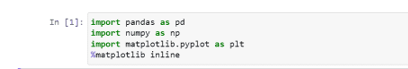
Let us import the required libraries first

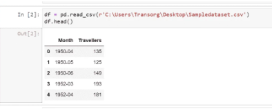
Now, let us read our dataset using the pandas library. Our dataset is in the form of a CSV (comma-separated values) file:

Now, I’m checking the datatype of the features present in the dataset:

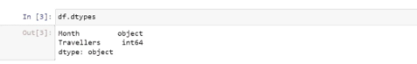
We found that the feature ‘Month’ is of the object type. So, we need to change it to datetime. Before that, let us check the missing values in the dataset:

Checking if there are any null values in the dataset:

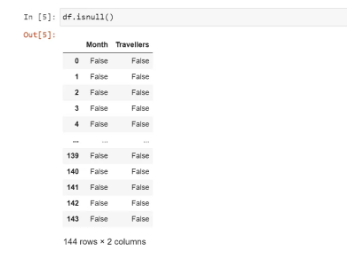
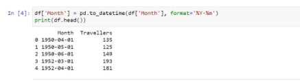
We found that there are no null values in the dataset. So, we changed the datatype of ‘Month’ to datetime:

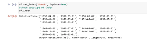
After performing the data preprocessing and changing the data types, we now need to convert our dataset to the time series data:

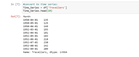
Next, we are going to visualise our time series data:

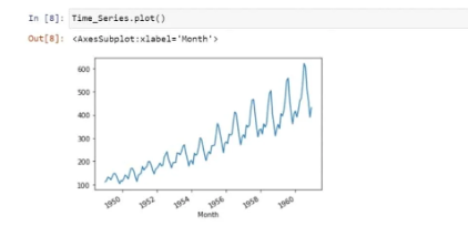
We have seen that there is a positive trend along with some seasonality in it. We are now checking for stationarity as it is an important step in the Time Series Analysis:

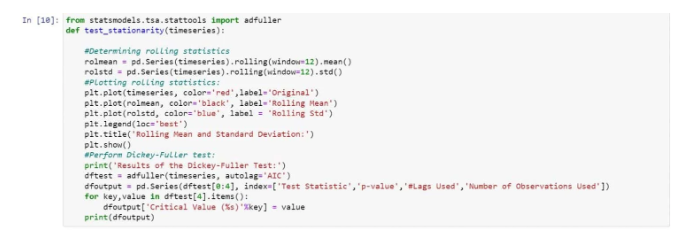
We have used a dickey-fuller test to check the stationarity. The Dickey-Fuller test is a type of statistical test used to check stationarity in the data:

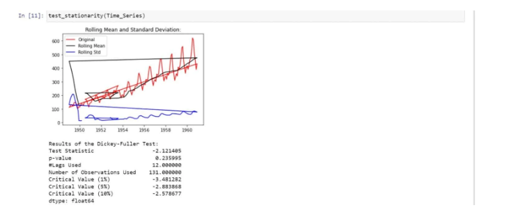
We found that there is no stationarity in the data due to the following reasons:

• The mean is increasing even though the standard deviation is small.
• Test Statistics is greater than the critical value.

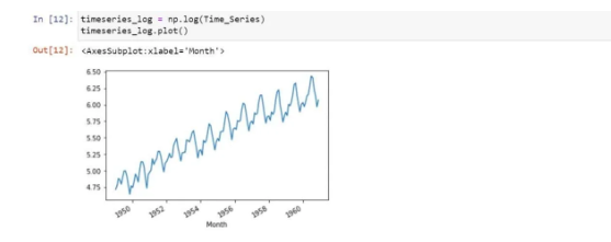
So, in order to make it stationarity, we are using logarithmic transformation:

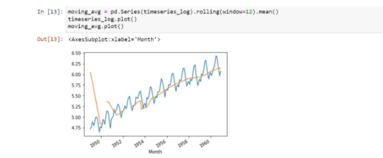
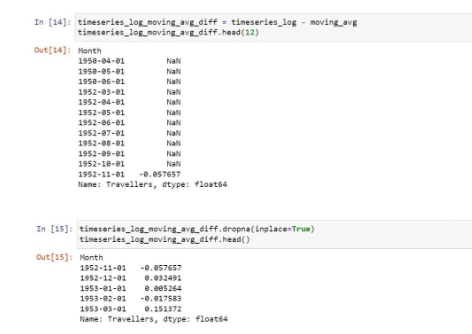
We found a positive or forward trend. In order to remove them, we are using the smoothing method. So, let’s use the moving averages method which is a type of smoothing method:

So, now we need to subtract the rolling mean from the original data.

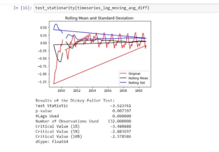
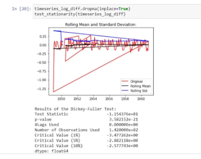
Now, let’s parse it to check for stationarity:

In the graph, we observe that there is no specific trend and even the test statistics is smaller than the critical value of 5%. That means, we can say it is stationary:

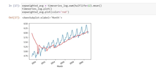
In the above process, we took an average of 12 months. But, sometimes, we need to work with a more complex range. The parameter (halflife) is assumed to be 12. Let’s check stationarity now/

We found that the above is stationary because the mean and standard deviation have fewer variations. At the same time, the test statistic is smaller than the 1% critical values

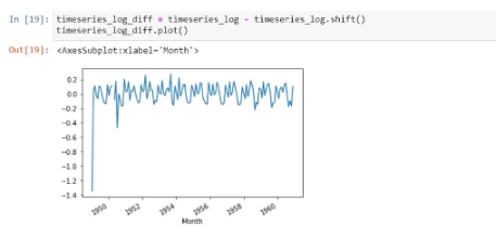
Let’s do the differencing now:

The above looks fine!

So, now just decompose the data into the components of time series. Here we model both the trend and the seasonality, and then the remaining part of the time series is returned:

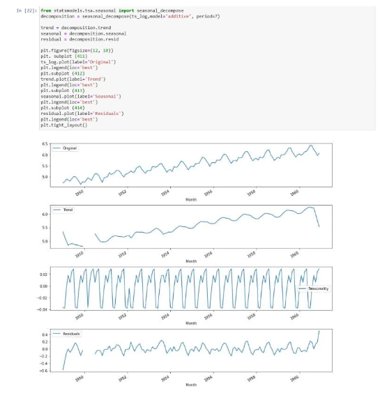
We can now use the residual values after removing the trend and seasonality from the time series. Check stationarity now:

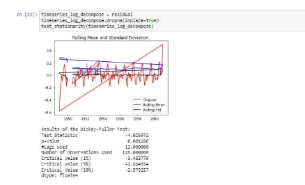
The above is stationarity because the test statistic is less than the critical values and the mean, and standard deviation has very few variations with respect to time.

At last, we are visualising the autocorrelation:

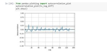
We have seen how to change the original data to time series and checking for stationarity, etc., using python. So, time series analysis in python makes it easy to analyse the time series data without any hassles.

Conclusion

Almost every Data Scientist will have to perform time series data analysis at some point in their career. Data Scientists can find trends, foresee occurrences, and subsequently guide decision-making by having a solid understanding of the tools and methodologies for analysis.

Promotional planning can be made more profitable for businesses by using stationarity, autocorrelation, and trend decomposition to understand seasonality patterns.

In conclusion, using time series forecasting to foresee future events in your time series data can have a big influence on decision-making. Any Data Scientist or Data Science team looking to use time series data to add value to their business will find these kinds of analyses to be extremely helpful.

I hope you enjoyed the blog. Now, it’s your time to implement the Time Series Analysis!

Frequently Asked Questions

Can I use deep learning for Time Series Analysis in Python?

Yes, deep learning can be effectively used for Time Series Analysis. Libraries like TensorFlow and Keras provide tools for building neural networks, including recurrent neural networks (RNNs) and long short-term memory (LSTM) networks, which are particularly suited for sequential data.

These models can capture complex patterns and dependencies in time series data, often outperforming traditional methods on large datasets.

How can I Visualise Time Series Data in Python?

Visualising time series data is essential for understanding trends and patterns. You can use libraries like Matplotlib and Seaborn to create line plots, scatter plots, and heatmaps. For example, you can use plt.plot() from Matplotlib to plot the time series data against time.

Additionally, libraries like Plotly and Bokeh offer interactive visualisations that can enhance data exploration.

What is the Difference Between ARIMA and Seasonal ARIMA (SARIMA)?

ARIMA (AutoRegressive Integrated Moving Average) is a popular model for forecasting non-seasonal time series data. It combines autoregression, differencing, and moving averages.

SARIMA extends ARIMA by including seasonal components, making it suitable for time series data with seasonal patterns. SARIMA incorporates seasonal differencing and seasonal autoregressive and moving average terms, allowing it to model seasonal effects effectively.