What Is VLOOKUP in Excel, and How Does It Work?

Summary: VLOOKUP in Excel is a powerful function for searching and retrieving data from large datasets. It simplifies data matching, financial analysis, and inventory tracking. Understanding its syntax, common errors, and alternatives like INDEX-MATCH enhances accuracy and efficiency, making Excel data management faster and more effective for users of all levels.

Introduction

Excel functions are powerful tools that enhance data management, making it easier to analyse and manipulate information. One of the most widely used functions is VLOOKUP in Excel, which helps users quickly search for specific data within large datasets. 

This blog aims to explain how VLOOKUP in Excel works, providing a clear understanding of its syntax, usage, and practical applications. By the end, you’ll grasp the essential aspects of this function, learn to avoid common errors, and discover how VLOOKUP can streamline tasks like data matching, analysis, and reporting for better decision-making.

Key Takeaways

• VLOOKUP in Excel simplifies data retrieval by searching for values in a dataset’s first column.
• Syntax includes lookup_value, table_array, col_index_num, and range_lookup for accurate searches.
• Common errors like #N/A, #REF!, and #VALUE! occur due to incorrect data, missing values, or wrong column references.
• Alternatives like INDEX-MATCH provide more flexibility by allowing lookups in any direction, unlike VLOOKUP.
• VLOOKUP is helpful for financial analysis, data comparison, and inventory tracking across various industries.

What Is VLOOKUP?

VLOOKUP, short for “Vertical Lookup,” is a powerful Excel function used to search for a specific value in the first column of a table or range and return a value from a different column in the same row. It simplifies Data Analysis by allowing users to quickly cross-reference and retrieve data from large datasets. 

For example, if you need to find an employee’s name by their ID number, VLOOKUP can search the employee ID column and return the corresponding name from another column.

Basic Structure and Syntax

The VLOOKUP function follows this basic syntax

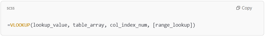
• lookup_value The value you want to search for in the first column of the table. This can be a number, text, or cell reference.
• table_array The range of cells that contains the data you want to search. It should include the column with the lookup value and the column from which you want to retrieve data.
• col_index_num The column number (starting from 1) within the table_array to return the value.
• [range_lookup] Optional. Use TRUE for an approximate match or FALSE for an exact match.

This structure enables VLOOKUP to efficiently search, retrieve, and display relevant data based on your requirements.

How Does VLOOKUP Work?

To fully grasp how VLOOKUP works, let’s break down its parameters and see it through an example.

lookup_value

This is the value you want to search for in the first column of your table. It can be a specific number, text, or a reference to a cell containing the value you want to look up.

Example If you’re searching for a product code, the product code is your lookup_value.

table_array

The table_array is the range of cells containing the data you want to search through. The first column of this range must contain the lookup_value, while other columns can contain the values you wish to return.

Example If you’re working with product information, the table_array might include the product code and corresponding product names, prices, or other attributes.

col_index_num

The col_index_num specifies the column number (from the left) in the table_array that contains the data you want to retrieve. For instance, if the second column has the data you want, the col_index_num would be 2.

Example If you’re looking for the price of a product in the second column of your table, you would set the col_index_num to 2.

range_lookup

The range_lookup parameter determines whether you want an exact or approximate match. If TRUE (or omitted), VLOOKUP will find an approximate match. If FALSE, it will only return an exact match.

Example If you want an exact price, you will use FALSE to ensure VLOOKUP searches for an exact match to the lookup_value.

Step-by-Step Example of a VLOOKUP Function

Let’s consider a table with product codes and corresponding product names and prices. You want to find the price of a product given its product code.

Here’s how you would write the VLOOKUP function

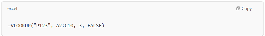
Explanation

• “P123” is the lookup_value — the product code you’re searching for.
• A2C10 is the table_array — the range where your product data is stored, with product codes in column A, names in column B, and prices in column C.
• 3 is the col_index_num — the column number where the price is located (column C).
• FALSE indicates that you want an exact match for the product code.

In this example, VLOOKUP searches for the product code “P123” in the first column of the table (A2A10). Once it finds the match, it returns the corresponding value from the third column (column C), the product’s price.

Common Use Cases for VLOOKUP

VLOOKUP is a versatile function that can streamline several data-related tasks. It’s beneficial when managing large datasets, allowing users to retrieve information, match values, and perform comparisons quickly. Here are a few key areas where VLOOKUP shines

Data Matching and Comparison

VLOOKUP is commonly used to match data from different tables. For example, you can compare customer lists or sales records by matching customer IDs, product names, or invoice numbers. This helps ensure consistency and accuracy across datasets without manually scanning for discrepancies.

Financial Analysis

In financial analysis, VLOOKUP helps link financial data across various reports. You can use it to pull financial figures from a general ledger into a summary report, making the analysis process more efficient. VLOOKUP also aids in budgeting, forecasting, and tracking financial performance by quickly pulling in relevant figures like expenses, revenue, or account balances.

Inventory Management

VLOOKUP is a powerful tool for inventory management. By linking product IDs with stock quantities, suppliers, and pricing information, VLOOKUP makes it easier to track inventory levels in real time. For example, it can quickly update stock levels in an inventory spreadsheet or pull up supplier details based on product IDs, ensuring seamless inventory tracking and management.

VLOOKUP saves time and improves accuracy by automating data retrieval and reducing manual effort in all of these use cases.

Common Errors in VLOOKUP

VLOOKUP is a powerful function in Excel, but like any tool, it can produce errors if used incorrectly. Understanding these common errors is essential for troubleshooting and ensuring the accuracy of your results.

#N/A Error

The #N/A error in VLOOKUP occurs when the function cannot find the lookup value in the specified range. This typically happens when

• The lookup value is misspelled.
• The value does not exist in the table array.

Example

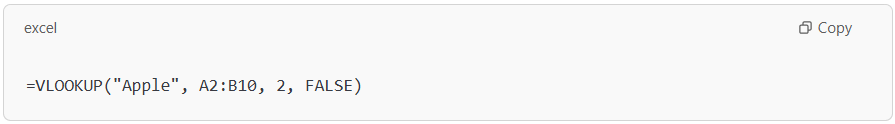
Troubleshooting Tip Double-check the lookup value for accuracy, ensuring it exists in the first column of the lookup table.

#REF! Error

A #REF! error occurs when the column index number in the VLOOKUP formula refers to an invalid column. This usually happens if you delete a column or change the table structure.

Example

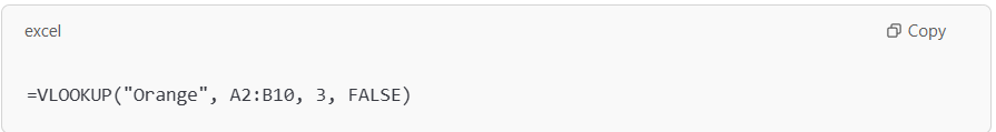
Troubleshooting Tip Ensure the column index is within the range of columns in your table array. Adjust the column index if necessary.

#VALUE! Error

This error occurs when one of the arguments in your VLOOKUP function is of an invalid type, such as using text where a number is expected or vice versa.

Example

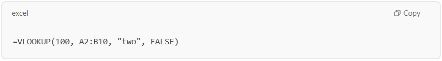
Troubleshooting Tip Make sure all arguments in the formula are of the correct type (numbers, text, etc.).

Incorrect Range Lookup (TRUE/FALSE)

The fourth argument in VLOOKUP determines whether to use an approximate match (TRUE) or an exact match (FALSE). Using TRUE when you expect an exact match can cause unintended results.

Example

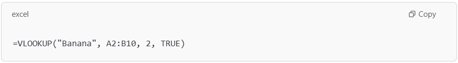
Troubleshooting Tip Always use FALSE for exact matches to avoid unexpected results.

By understanding and troubleshooting these common errors, you can enhance the reliability of your VLOOKUP functions and avoid common pitfalls.

Alternatives to VLOOKUP

VLOOKUP is a powerful tool in Excel, but it’s not always the best fit for every task. For users who need more flexibility or efficiency, other functions can handle lookup operations more effectively. Two common alternatives to VLOOKUP are HLOOKUP and the combination of INDEX-MATCH.

HLOOKUP

HLOOKUP (Horizontal Lookup) is similar to VLOOKUP but is used when the data you need to search through is organised horizontally rather than vertically. While VLOOKUP searches columns, HLOOKUP searches rows. This makes it a great choice when working with data arranged across multiple rows.

Example

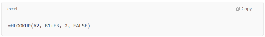
This function looks for the value in cell A2 across the first row of the range B1F3 and returns the corresponding value from the second row. HLOOKUP can be handy in situations where data is structured more horizontally.

INDEX-MATCH

Combining INDEX and MATCH provides a more powerful and flexible alternative to VLOOKUP. INDEX returns a value based on its position within a range, while MATCH finds the position of a value in a row or column. Together, they allow for dynamic lookups in both horizontal and vertical data.

Example

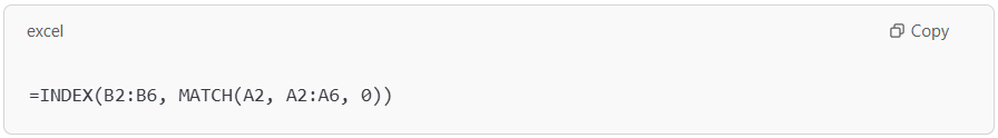
Here, MATCH finds the row number of A2 in the range A2A6, and INDEX returns the value from the same row in the range B2B6. This method is often preferred because it doesn’t require the lookup value in the first column (like VLOOKUP) and can look in any direction.

Both HLOOKUP and INDEX-MATCH offer more versatility than VLOOKUP, making them excellent tools for users needing advanced Excel data management.

Closing Statements

VLOOKUP in Excel is an essential function that simplifies data retrieval, enhances efficiency, and streamlines analysis. By understanding its syntax, parameters, and common errors, you can leverage it for data matching, financial analysis, and inventory management. While VLOOKUP is powerful, alternatives like HLOOKUP and INDEX-MATCH offer more flexibility. 

Mastering VLOOKUP improves accuracy and saves time when handling large datasets. Learning this function will enhance your productivity whether you’re a beginner or an advanced Excel user. By avoiding common pitfalls and choosing the right lookup method, you can make data management seamless and more efficient in everyday tasks.

Frequently Asked Questions

How Do I Use VLOOKUP in Excel for Exact Matches?

To use VLOOKUP for exact matches, set the last parameter to FALSE. Example =VLOOKUP(1001, A2C10, 2, FALSE). This ensures that Excel only returns results that perfectly match the lookup value in the first column of your dataset.

Why is My VLOOKUP Returning an #N/A Error?

An #N/A error occurs when the lookup value isn’t found in the first column of the table array. Check for typos, incorrect cell references, or mismatched data formats. Ensuring the lookup column is sorted correctly and contains the exact value format will help resolve this issue.

What is The Difference Between VLOOKUP and INDEX-MATCH?

VLOOKUP only searches from left to right, requiring the lookup column to be the first column. INDEX-MATCH is more flexible, allowing lookups in any direction. INDEX-MATCH is also faster in large datasets, making it a better alternative for complex searches.